Intelligent complex for modeling safety movement of a multi-agent group of marine robots in uncertain environments

Intensive development today is observed in the areas of data processing and analysis, as well as in the management of robotic systems; Artificial Intelligence (AI) systems are increasingly used. As the complexity of the tasks facing the Marine Robotic Complex (MRC) increases, the need for the use of AI technologies becomes clear. These technologies provide safe movement and control of marine objects, navigation of MRC in maritime space, development of behavior logic in unknown environments and planning of their movement, as well as optimization of data processing. The development of MRC currently covers various areas for which there is no single solution yet. This article outlines the development process of a simulation complex designed to model an intelligent system (IS) for strategizing the motion of a collective of marine robotic systems. It includes an in-depth exposition of individual modules and the mathematical modeling of the employed algorithms.

Introduction

At present, intelligent systems enjoy a wide array of applications owing to progress in AI technology, which amplifies human abilities and proficiencies.

Artificial Intelligence (AI) is commonly employed today to describe applications handling intricate tasks that were previously exclusive to humans. AI enables the replication and enhancement of our learning from the surrounding environment and the utilization of such information. This aspect of AI serves as the foundation for innovation. AI relies on diverse machine learning technologies that identify data patterns and formulate predictions. Given this characteristic, AI serves as an intermediary or often intersects with multiple technologies, thereby enhancing the potential of the utilized system and achieving optimal results more efficiently.

In the contemporary era, AI, ML (Machine Learning), and DL (Deep Learning) technologies are extensively applied within the realm of marine robotics. These methodologies are increasingly employed by developers for the deployment of planning systems, control mechanisms, and internal diagnostic systems across various types of robotic platforms, including airborne [1,2], terrestrial [3,4], and marine robotic systems [5-7], encompassing underwater gliders, surface gliders [8-10], and for tasks such as monitoring and patrolling potentially hazardous underwater entities. Intelligent systems facilitate adaptation to uncertain environments, enabling the execution of goal-setting functions and action planning for aerial, terrestrial, and maritime robotics [11-14].

In marine robotics, artificial intelligence technologies are widely used in the field of docking underwater vehicles [15-17], in the system of planning the movement of single ANPA and their groups [18-22]. Artificial intelligence technologies are also increasingly being used in vision systems. They allow the ANPA to identify various objects in the water space [23-26], detect damage at underwater infrastructure facilities [27-30], and much more [31-35].

Reinforcement learning techniques are extensively employed in motion planning systems for both individual robots and their collectives [36-41]. However, existing findings from relevant research and literature predominantly discuss the utilization of Artificial Neural Networks under specific deterministic circumstances, where predetermined values for the operational environment are known. Additionally, these sources highlight the use of centralized AI systems to optimize the allocation of robot groups across an area and facilitate group coordination to address overarching objectives (e.g., employing the smart factory model) [19]. Many methodologies rely on analyzing data from pre-existing maps, a resource typically unavailable in real-world conditions.

The analysis conducted indicates that existing methods and algorithms are currently unable to directly address the challenges associated with monitoring, patrolling, and surveilling specific territories and objects. These objects include potentially hazardous underwater entities

Our study introduces a novel algorithm that integrates graph-analytical and neural network methodologies. This combination of reinforcement learning and graph-based algorithms offers several advantages, allowing robotic complexes and their groups to swiftly identify potential research areas and leverage acquired knowledge to maximize rewards. For instance, graph-based algorithms can compute global situations, trajectories, and future states of individual robots or groups, which may yield high rewards, along with optimal strategies for state changes. Reinforcement learning can then utilize this information to enhance performance.

In the presented article, we address the formal statement of the problem and challenges related to utilizing the MRC group in environments with uncertainties and obstacles.

The use of intelligent planning systems for the formation of trajectories of movement of groups of marine robots should significantly increase the safety of navigation, and eliminate the occurrence of emergencies in conditions of passage of narrow nesses, channels, and other previously unknown dynamic obstacles encountered in the water area.

The presented article has the following structure. The first section describes the development of an algorithm for forming a group interaction area. The second section is devoted to the development of an algorithm for a single group visibility field. The third section describes the development of a global planning module and the architecture of a unified neural network multi-agent group interaction system. The process of modeling this system is presented.

In conclusion, the main results obtained during the work and the direction of further research are described.

Section 1. The problem statement

Employing MRC groups in genuine maritime settings invariably demands the utilization of high-precision technologies to guarantee accurate positioning and essential parameters for radio and hydroacoustic communication. Nevertheless, developers often encounter challenges in accounting for diverse indicators of marine environmental stratification, the existence of multidirectional currents, and other non-stationary processes, particularly when MRCs are deployed in 3D marine environments. Striving for precision in the application of MRC groups results in the intricacy of algorithm development, and conversely, in the complexity of implementation and application under real-world conditions.

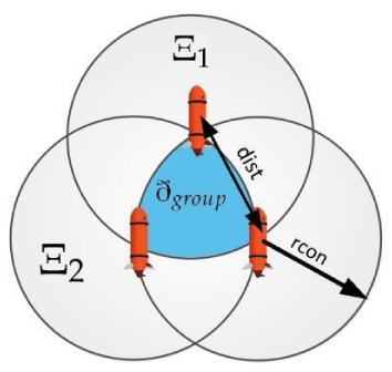
As a result, the authors of the paper opted to depart from the conventional approach of constructing a “hard-coded system” for forming MRCs and instead adopted a method based on AGI (the Area of Group Interaction). This method can be outlined by the following parameters (when applying the algorithm in a 2D context) (1):

$\begin{array}{l}{\text{þ}}_1={\Xi }_1{{\displaystyle \cap }}^{\text{}}{\Xi }_2\hfill \\ {\text{þ}}_2={\text{þ}}_1{{\displaystyle \cap }}^{\text{}}{\Xi }_3\hfill \\ {\text{ þ}}_{group}={\text{þ}}_1{{\displaystyle \cap }}^{\text{}}{\text{þ}}_2\hfill \end{array}\text{ (1)}$

where ${\Xi }_1(r_{co{n}_1},dis{t}_r),{\Xi }_2(r_{co{n}_2},dis{t}_r),{\Xi }_3(r_{co{n}_3},dis{t}_r)$ The operational boundaries for each agent within the group are determined by considering the distance between agents and the permissible communication range.

An illustration depicting the formation of the AGI is provided in Figure 1.

Figure 1: Depicting the formation multi-agent marine system based on AGI.

The resulting values following the execution of the algorithm consist of the variables, $[R,E_{dist},E_{con}]\in {\text{þ}}_{group}$ . which characterize the relationships among all agents within the group (2)

$\begin{array}{l}{E}_{dist}=\left[\begin{array}{l}|R_1-R_2|-dis{t}_r\hfill \\ |R_1-R_3|-dis{t}_r\hfill \\ |R_2-R_3|-dis{t}_r\hfill \end{array}\right]E_{con}=\left[\begin{array}{l}{r}_{con}-|R_1-R_2|\hfill \\ r_{con}-|R_1-R_3|\hfill \\ r_{con}-|R_2-R_3|\hfill \\ \hfill \end{array}\right]\hfill \end{array}\text{ (2)}$

The provided set of parameters is utilized for the subsequent training of the group neural network, tasked with analyzing and providing recommendations for future actions, either as a single agent within the group or for the group as a whole.

Section 2. Development of an algorithm group field of view (GFOV) for a multi-agent marine system

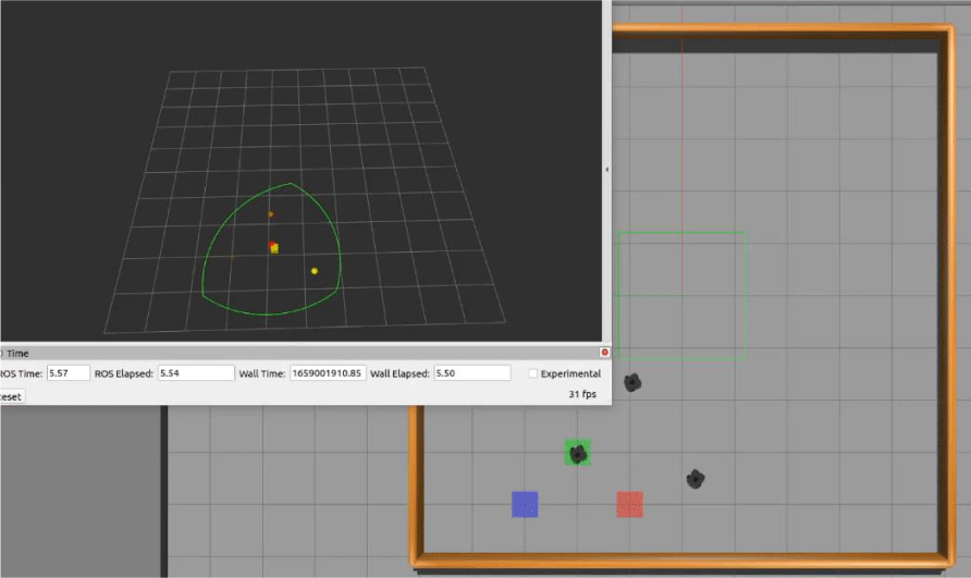
To simulate the operation of the Visual System (VS), we employed the Astra Pro Realsense camera model, which is compatible with ROS (Robot Operating System). During operation, the depth camera generates an array of points with a resolution of 640 x 320, resulting in 204800 points. These points are converted into the PointCloud2 type and then transmitted to the Rapidly-exploring Random Tree (RRT) module. To enhance processing speed, it is feasible to decrease the resolution of the depth camera. The GFOV module receives a PointCloud2 data set consisting of 204800 * N points from the Realsense camera (where N- count of the agent in the group). Figure 2 illustrates an example of obtaining images from the camera.

Figure 2: Demonstrating the functionality of the neural network within the Visual System module for classifying 2 class visible objects.

Utilizing data from the sensory system, the agent can gather information about the surrounding environment. VS comprises two primary functional modules: the obstacle detection module and the object identification module. The object identification module is responsible for recognizing objects within the agent’s field of view and serves as a supplementary component, providing additional data to the Autonomous Vehicle’s (AV) neural network. For simplification, only two classes were defined: “obstacles” and “agents”.

The task of class distribution is handled by the YOLOv5 pre-trained neural network, proficient in resolving such tasks. This neural network is trained on user data by incorporating an additional dataset containing predefined “obstacles” and “agent” areas.

As this work focuses on the design of a planning system for a 2D setting, readily available TurtleBot3 models with predefined action sets were utilized to streamline the development of a software simulation complex.

Consequently, a software simulation complex was developed based on the ROS framework, incorporating its Gazebo and RVIZ software components. The collected dataset comprises simulated group motions of TurtleBot3 Autonomous Vehicles (AVs) and a camera mounted on their platform, as depicted in Figure 2.

Additionally, a dataset containing 270 images has been compiled, where specific 2 class “obstacles” and “neighboring agents” have been delineated and appropriate labels assigned. Training was conducted using the following parameters:: epoch = 500, batchsize = 16.

Section 3. Development of a simulation complex for intelligent modeling

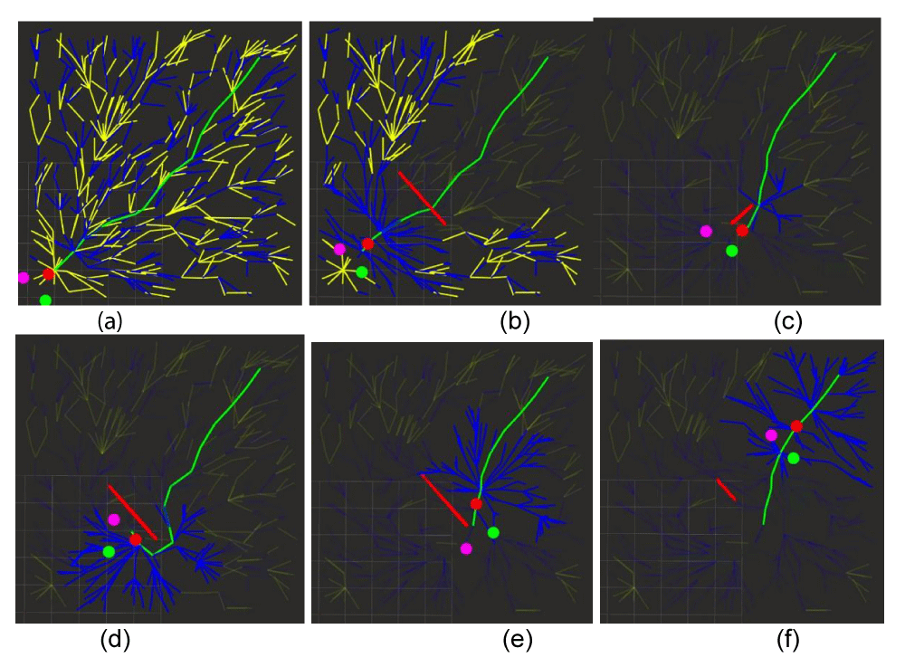
The devised system for global trajectory planning relies on the real-time RRT* method. The main objective of the MRC group is to navigate from the initial point to the destination. To achieve this, the proposal suggests constructing a map of random tree branches that span the entire designated area. This procedure is efficient and can be conducted before launch. The authors have previously conducted thorough investigations and adjustments of this algorithm for application in the realm of marine robotics [40-42].

Utilizing the internal libraries ROS framework, the points obtained from the Visual System are recalibrated, considering both the heading angle and the global coordinate system. In the application of the RRT algorithm, the proximity of graph points to obstacle points is assessed, resulting in the blocking of inaccessible graph points.

An illustration of the algorithm’s functionality is depicted in Figure 3, showcasing a group of robots in motion.

Figure 3: Multi-agent group RRT* simulates ( (a) - in motion process, (b,c) - obstacle detection process, (d-e) - bypassing an obstacle).

The proposed method of forming interaction of a group of robots allows the exchange of data using vision systems between agents in the group. The global planning module, informed by the GFOV module, establishes a comprehensive motion trajectory. The AGI generation module facilitates the selection of optimal paths for group reconfiguration and obstacle avoidance, considering the required communication distance between agents.

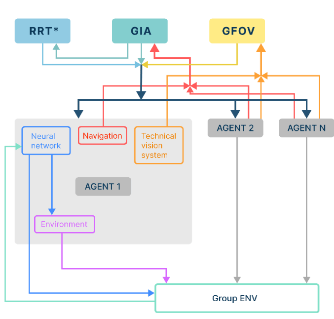
The structure of the newly created intelligent planning system, taking into account both input and output parameters, is depicted in Figure 4. To produce control signals for the actuators of each group member, an internal planning logic has been incorporated. This logic relies on an artificial neural network and employs deep learning techniques tailored to each agent.

Figure 4: Architecture of intelligent path-planning system for the multi-agent MRC (GFOV – group field of view, GIA – group interaction area).

The operation of an algorithm, based on the cascade intelligent planner illustrated in Figure 4, unfolds as follows: The GPOV, GIA (group interaction area (the same as AGI), and RRT* modules receive input data from the navigation systems and Visual Systems (VS) of each agent within the group. As explained earlier, the output of the GPOV operation is an array of data describing the current status of the shared field of view, including object classifications. The AGI algorithm provides data on the current state of the formation as εn and D. Additionally, the auxiliary trajectory planning module computes the recommended trajectory in the form of H_group. This dataset is then forwarded to the neural system responsible for path planning for each agent within the group, governing the actions of each agent during learning. Consequently, each agent operates within its environment (the agent’s local environment Eagent), from which it receives feedback in the form of an updated state S′ and the reward R. Simultaneously, the agent remains in constant interaction with other agents within the group, meaning its local environment is an integral part of the overall group environment Eagent ∈ E_group.

As a result, there is an easily implemented and scalable decentralized group planning system. Such a system implements algorithms, which provide the preparation and generation of data for the onboard agent’s neural network training.

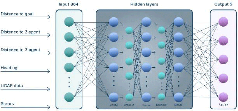
The architecture of the neural network is shown in Figure 5.

Figure 5: Neural network architecture.

The neural network comprises 364 input values, encompassing arrays representing distances between group agents, the distance and directional angle of the current agent relative to the target, as well as data from the Visual System, the identifier of detected objects (obstacles or group agents), and the current status of the agent. This information feeds into the internal block of the neural network, which consists of three dense layers, each containing 64 neurons, along with two dropout layers featuring an exclusion parameter of 0.2. The RMSProp optimizer is employed, with parameters set as follows: learningrate = 0.00025, ρ = 0.9, ε = 1⁻⁶, serving as the activation function.

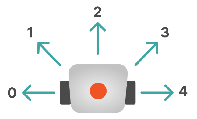
The previously established software simulation complex was utilized as the training environment. Interaction between the agent and the environment is facilitated through five potential actions, outlined in Figure 6.

Figure 6: Agent’s actions.

During interaction with the environment, the Autonomous Vehicle (AV) transitions from state (S) to state (S′) based on a specific reward (R). The expression defining the internal policy responsible for the AV’s reward function is as (3):

$\begin{array}{l}{R}_r=Y_r(A)\text{*}5\text{*}{D}_{\text{rate}}\hfill \\ D_{\text{rate}}=2^{D_{\text{cur}}/D_{\text{goal}}}\hfill \\ Y_r(A)=1-4|0.5-0.5\text{*}\alpha |\hfill \\ \alpha =\text{heading}\hfill \end{array}\text{ (3)}$

Here, “heading” represents the current direction of the agent. D_rate and Y_r(A) denote the components of the reward derived from the distance and the agent’s current heading, respectively. D_goal - represents the distance between the agent and the target

The neural network correction module for planning the actions of the MRC group is tasked with assessing the actions executed by each agent within the group. The principal aim of this module is to establish an intragroup behavior policy by analyzing the states and rewards (S_n, R_r, n) for all agents within their local environment Eagent and the collective group environment E_group..

The neural network correction module for planning actions of the MRC group is responsible for evaluating the actions performed by each agent in the group. The primary objective of this module is to form an intragroup policy of behavior through the analysis of states and rewards for all agents in local and overall group environments.

The expression defining the policy of intragroup interaction among agents, which governs the formation of the group reward component, is as (4-6):

$R_{g13}=\{\begin{array}{ll}-e^{D_{13}-2.1}\hfill & \text{if}{D}_{13}<2.1\hfill \\ -e^{1.9-D_{13}}\hfill & \text{if}{D}_{13}<1.9\hfill \\ 3\hfill & \text{othercases}\hfill \end{array}\text{ (4)}$

$R_{g12}=\{\begin{array}{ll}-e^{D_{12}-(\sqrt{2}+0.1)}\hfill & \text{if}{D}_{12}>\sqrt{2}+0.1\hfill \\ -e^{(\sqrt{2}-0.1)-D_{12}}\hfill & \text{if}{D}_{12}<\sqrt{2}-0.1\hfill \\ 3\hfill & \text{othercases}\hfill \end{array}\text{ (5)}$

$R_{g1}=R_r+R_{g12}+R_{g13}\text{ (6)}$

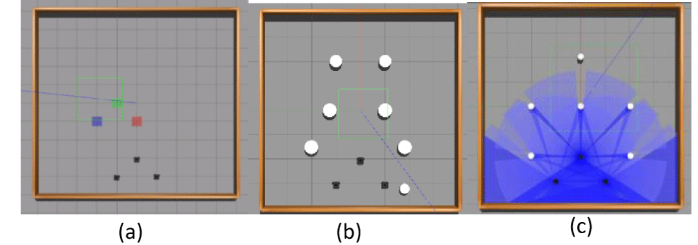
To train a group of three agents, various scenarios were simulated in the software simulation complex, including scenarios without obstacles, with stationary obstacles, and with dynamically changing obstacles. These scenarios are depicted in Figure 7. It is important to highlight that during this stage, the initial structure of the wedge-type formation was employed.

Figure 7: The scenes created are designed to facilitate simulations within the motion planning neural system for the group of objects: (a) - stage without obstacles; (b) - scene with static obstacles; (c) - scene with dynamic obstacles.

The training was carried out on a PC featuring an NVIDIA GeForce 3060 graphics card with 12 GB of RAM (utilizing pre-installed CUDA 11.7), 64 GB of DDR4 RAM, and an Intel Core i9 processor running at 4.016 GHz. The duration of training varied for each scene: approximately 2 hours for the first scene, 10 hours for the second scene, and around 15 hours for the third scene.

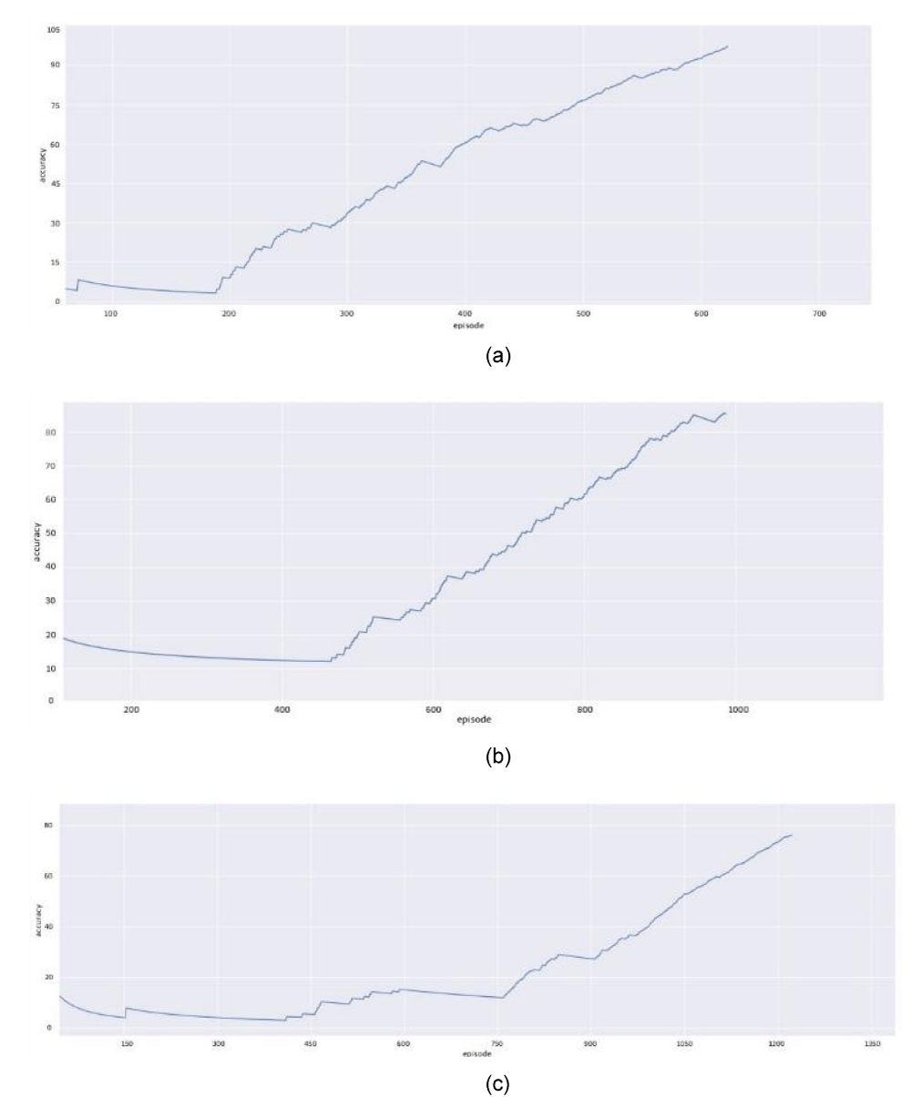
The graphs depicted below in Figure 8 illustrate the learning outcomes for the three generated scenes. Additionally, an instance of training a group within a scene devoid of obstacles, yet incorporating the AGI display and its alterations throughout the motion, is depicted in Figure 9.

Figure 8: The learning outcomes of the path-planning multi-agent neural network system for the MRC group are as follows: (a) - Total score plot depicting the group’s performance in a scene without obstacles. (b) - Total score plot illustrating the group’s performance in a scene with obstacles. (c) - Total score plot indicating the successful mission completion in a scene with moving obstacles.

Figure 9: An illustration showcasing the changes in AGI during the simulation of object group motion within an obstacle-free environment.

In Figure 8, plots (a) depict the outcomes of group training in an obstacle-free environment. As evidenced by the figures, the developed group neural network effectively manages (with a 90% probability) accident-free group motion after 400 training epochs (episodes), while adhering to the conditions stipulated by the AGI and shared field of view algorithms to attain the target coordinates.

Plots (b) and (c) illustrate the results of group training in environments featuring static and dynamic obstacles, respectively. Following 800 epochs (episodes) of training, the neural network adeptly navigates (with a 75% probability) the group motion to reach the target coordinates, all while evading obstacles.

The peculiarity of the functioning of UUV and MRC is their movement in a non-deterministic environment, in which complex hydrodynamic conditions, such as dynamic water flows caused by various factors, tides, wind forces, and other geographical features, can have a significant impact on the movement of the vessel.

Modern UUV planning and control systems must take into account complex hydrodynamic conditions to ensure reliable and safe movement. Consideration of the impact of currents on navigation becomes extremely important in the context of the growing number of offshore vessels, where the vessel is controlled completely autonomously in real-time. Thus, the lack of information about currents in the water area where the UUV operates can lead to non-optimal routes, increased energy consumption, and the risk of emergencies.

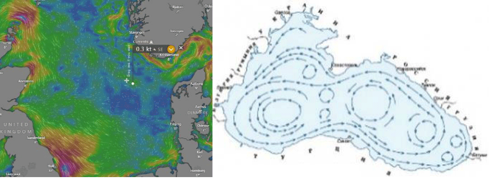
As a rule, current maps are an image that shows the directions of currents characteristic of the region in question. In this case, surface currents are considered, which can be described by two parameters, intensity and direction.

Let us denote the field of currents by ϱ and ξ , which describe the parameters of intensity and direction, respectively. Figure 8 shows examples of such maps for the White and Black Seas.

From the data presented on the maps, one can judge the parameters of the direction and intensity of currents. Figure 10 shows the intensity and direction of the current at the selected point (0.3 knots and SE direction).

Figure 10: Map of flow Black and White Sea.

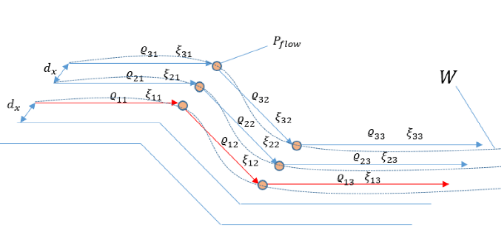
The description of the current field can be provided by a set of nodal points (7):

$x = [x_i,x_{i+1},\mathrm{...},x_{k-1},x_k]\text{ (7)}$

$y = [y_i,y_{i+1},\mathrm{...},y_{k-1},y_k]$

Where i = 1..k, K– finite number of spline points N_i,k(x). b-spline is used as a function limiting the flow zone W. General formula for calculating b-spline coefficients (8):

$N_{i,k}\left(x\right)=\frac{x-t_i}{t_{i+k-1}-t_i}{N}_{i,k-1}\left(x\right)+\frac{t_{i+k}-x}{t_{i+k}-t_{i+1}}{N}_{i+1,k-1}(x)\text{ (8)}$

Where I - is the index of the current point, x is the value from i to i+1 (step), t is an array of indices (9):

$\{\begin{array}{cc}0,& if i<k\\ i-k+1,& if k\le i\le n\\ n-k+2,& if i>n\end{array}\text{ (9)}$

Let us determine the values of intensity ϱ and direction ξ of the flow at each point χ( ϱ,ξ)∈W, as a deviation from the standard value (for example, Flow=5) as per the expression (10):

${\varrho }_{j1}=Flow*(1+△Q),j=1\text{ (10)}$

${\varrho }_{j1}={\varrho }_{(j-1)1}*K_{int},j=2$

Where ∆Q = [-0.1…0.1] is the coefficient of change in flow intensity, K_int = 0.3 is the coefficient describing the gradient of change in flow intensity from ϱ11 to ϱj1 (11).

$Q=\left[\begin{array}{ccc}{\varrho }_{11}& \cdots & {\varrho }_{j1}\\ ⋮& \ddots & ⋮\\ {\varrho }_{1k}& \cdots & {\varrho }_{jk}\end{array}\right]\text{ (11)}$

where j - is the number of splines defining the digital flow field, k- is the number of key points of the P_flow splines. It should be taken into account that ϱ_jk = const for all values of P_flow(j,k).

The flow direction ξ at each point X(ϱ, ξ) ∈ W can be described by the following expressions (12):

$\xi = \xi { }_i+△{С}_{\xi },$

$\xi { }_i= atan(△y_i/△x_i)\text{ (12)}$

$△y_i = y_i-y_{i-1}$

$△x_i = x_i-x_{i-1}$

Where x_i, y_i are the current points at which the direction of the current is calculated, ∆Cξ is the random component introducing error (non-deterministic impact/noise) in the range (0.3 ....0.3).

Thus, for any arbitrary point P_cur on the map of the water area, the intensity and direction parameters can be calculated taking into account expressions (8-12) taking into account the definition of two adjacent points X_i and X_i-1 (13):

${\xi }_{P_{cur}}=\frac{\xi { }_i-\xi { }_{i-1}}{2}$

${\varrho }_{P_{cur}}(j,k)= \frac{({\varrho }_{jk}- {\varrho }_{jk-1})}{2}\text{ (12)}$

A schematic representation of the flow field construction is presented in Figure 11.

Figure 11: Scheme for constructing a flow field.

The resulting model of the characteristic current map can be used in the module for planning the global trajectory of a multi-agent group MRC and introducing appropriate adjustments during the mission.

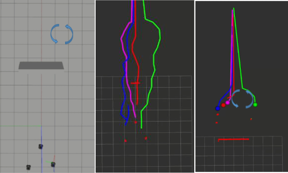
An example of taking into account a circular flow on a stage with a “wall” obstacle is shown in Figure 12.

Figure 12: An example of taking into account circular flow when moving in a scene with a “wall” obstacle.

As can be seen from the simulation results, the developed system ensures that a group of agents successfully bypasses detected obstacles.

It is important to note that the system effectively takes into account the complex structure of the current map, which can include both currents directed following the movement of a group of agents and currents opposite to the direction of movement of the group.

Conclusion

The article considered the process of developing an intelligent planning system for the movement of a group of marine mobile objects and the possibility of safely (accident-free) performing positional tasks related to monitoring and patrolling a given territory.

The proposed system relies on modules that integrate neural network methodologies and machine learning techniques, forming representations for the group’s field of visibility, intragroup interaction area, and an auxiliary global RRT* planner module.

The amalgamation of reinforcement learning algorithms and graph-based methods more effective exploration of potential solutions. This integration enables agents to navigate both deterministic and probabilistic environment policies, broadening the scope of solutions and ultimately enhancing performance. This combination proves advantageous over sole reliance on reinforcement learning, as it allows for a more comprehensive understanding of the environment and exploration of a wider array of solutions.

The available dataset supports deep learning for each agent’s neural network within the group. Additionally, continuous data exchange regarding the states of neighboring agents and subsequent analysis enables the implementation of a scalable and decentralized system structure for intragroup interaction. A supplementary policy for evaluating intragroup states involves exerting corrective influence on the training of the cascaded neural network action planner.

A software simulation complex has been developed based on ROS, RVIZ, Gazebo, and machine learning libraries, facilitating research on the developed models and planning methods. The simulation results showcase the efficacy of the proposed neural network planning algorithms.

All source code is written in Python, chosen for its ease of use and the availability of numerous auxiliary libraries. However, Python’s interpreted nature is considered slow. Once a fully functional prototype of the system is developed using full-scale models, there are plans to transition to C++ to enhance the system’s speed.

The methods and algorithms presented for group interaction, along with practical demonstrations, illustrate the potential use of the intelligent system within the Marine Robotic Complex (MRC) in a 2D environment. The existing architecture and modular principle of the planning system allow for further adaptation to utilize this system within Autonomous Underwater Vehicles (AUVs), considering the existing limitations and operational features of AUVs in a 3D environment.

Simulation modeling demonstrates a 90% probability of successful mission completion for group motion in obstacle-free environments and a 75% probability in environments with moving obstacles. An essential consideration is enhancing the neural network’s performance in environments containing obstacles, with the potential incorporation of convolutional layers into the agent’s neural network architecture.

A fundamentally new algorithm for constructing a characteristic model of the global current field is presented, taking into account the parameters of the intensity and direction of currents. The application of this algorithm in maritime navigation opens up new prospects for ensuring the safety and efficiency of ship movement in various hydrological scenarios. The model provides the ability to digitally predict currents, which allows ships to effectively choose optimal routes and minimize time costs. Vessels equipped with this algorithm can effectively navigate obstacles such as currents, wandering ice, and other hydrodynamic challenges with greater accuracy and anticipation. The developed model provides information on the intensity and direction of currents in narrows and channels, which significantly facilitates the navigation process and reduces the risk of collision.

1. Badrloo S, Varshosaz M, Pirasteh S, Li J. Image-Based Obstacle Detection Methods for the Safe Navigation of Unmanned Vehicles: A Review. Remote Sensing. 2022; 14. https://doi.org/10.3390/rs14153824.
2. Aslan MF, Durdu A, Yusefi A, Yilmaz AH. HVIOnet: A deep learning based hybrid visual-inertial odometry approach for unmanned aerial system position estimation. Neural Networks. 2022; 155:461-474. https://doi.org/10.1016/j.neunet.2022.09.001.
3. Ji Q, Fu S, Tan K, Thorapalli Muralidharan S, Lagrelius K, Danelia D, et al. Synthesizing the optimal gait of a quadruped robot with soft actuators using deep reinforcement learning. Robotics and Computer-Integrated Manufacturing. 2022; 78:102382.
4. Kouppas C, Saada M, Meng Q, King M, Majoe D. Hybrid autonomous controller for bipedal robot balance with deep reinforcement learning and pattern generators. Robotics and Autonomous Systems. 2021; 146. https://doi.org/10.1016/j.robot.2021.103891.
5. Gupta P, Rasheed A, Steen S. Ship performance monitoring using machine-learning. Ocean Engineering. 2022; 254. https://doi.org/10.1016/j.oceaneng.2022.111094.
6. Maevskij AM, Zanin VY, Kozhemyakin IV. Promising high-tech export-oriented and demanded by the domestic market 556areas of marine robotics. Robotics and technical cybernetics. 2022; 10(1):5-13. https://doi.org/10.31776/RTCJ.10101.
7. Sokolov SS, Nyrkov AP, Chernyi SG, Zhilenkov AA. The Use Robotics for Underwater Research Complex Objects. Advances in Intelligent Systems and Computing. 2017; 556:421-427. https://doi.org/10.1007/978-981-10-3874-7_39.
8. Silva Tchilian R, Rafikova E, Gafurov SA, Rafikov M. Optimal Control of an Underwater Glider Vehicle. Procedia Engineering. 2017; 176:732-740. Proceedings of the 3rd International Conference on Dynamics and Vibroacoustics of Machines (DVM2016) June 29-July 01, 2016, Samara, Russia. https://doi.org/10.1016/j.proeng.2017.02.322.
9. Tian X, Zhang L, Zhang H. Research on Sailing Efficiency of Hybrid-Driven Underwater Glider at Zero Angle of Attack. Journal of Marine Science and Engineering. 2022; 10. https://doi.org/10.3390/jmse10010021.
10. Wang P, Xinliang T, Wenyue L, Zhihuan H, Yong L. Dynamic modeling and simulations of the wave glider. Applied Mathematical Modelling. 2019; 66:77-9.
11. Beloglazov DA, Guzik VF, Kosenko EY, Kruhmalev V, Medvedev MY, Pereverzev VA, Pshihopov VH. Intelligent trajectory planning of moving objects in environments with obstacles. Moscow: Fizmatlit; 2014; 450.
12. Gul F, Mir I, Abualigah L, Sumari P, Forestiero A. A Consolidated Review of Path Planning and Optimization Techniques: Technical Perspectives and Future Directions. Electronics. 2021; 10. https://doi.org/10.3390/electronics10182250.
13. Kenzin M, Bychkov I, Maksimkin N. A Hierarchical Approach to Intelligent Mission Planning for Heterogeneous Fleets of Autonomous Underwater Vehicles. Journal of Marine Science and Engineering. 2022; 10. https://doi.org/10.3390/jmse10111639.
14. Shu M, Zheng X, Li F, Wang K, Li Q. Numerical Simulation of Time-Optimal Path Planning for Autonomous Underwater Vehicles Using a Markov Decision Process Method. Applied Sciences. 2022; 12. https://doi.org/10.3390/app12063064.
15. Sans-Muntadas A, Kelasidi E, Pettersen KY, Brekke E. Learning an AUV docking maneuver with a convolutional neural network. IFAC Journal of Systems and Control. 2019; 8:100049. https://doi.org/10.1016/j.ifacsc.2019.100049.
16. Wang Z, Xiang X, Guan X, Pan H, Yang S, Chen H. Deep learning-based robust positioning scheme for imaging sonar guided dynamic docking of autonomous underwater vehicle. Ocean Engineering. 2024; 293:116704. https://doi.org/10.1016/j.oceaneng.2024.116704.
17. Özdemir K, Tuncer A. Deep Reinforcement Learning Based Mobile Robot Navigation in Unknown Indoor Environments.
18. Neural network-based adaptive trajectory tracking control of underactuated AUVs with unknown asymmetrical actuator saturation and unknown dynamics. Ocean Engineering. 2020; 218:108193. https://doi.org/10.1016/j.oceaneng.2020.108193.
19. Li J, Du J. Command-Filtered Robust Adaptive NN Control With the Prescribed Performance for the 3-D Trajectory Tracking of Underactuated AUVs. IEEE Transactions on Neural Networks and Learning Systems. 2021:1–13. https://doi.org/10.1109/TNNLS.2021.3082407.
20. Fang K, Fang H, Zhang J, Yao J, Li J. Neural adaptive output feedback tracking control of underactuated AUVs. Ocean Engineering. 2021; 234:109211. https://doi.org/10.1016/j.oceaneng.2021.109211.
21. Sayyaadi H, Ura T. AUVS' Dynamics Modeling, Position Control, and Path Planning Using Neural Networks. IFAC Proceedings Volumes. 2001; 34. https://doi.org/10.1016/S1474-6670(17)35077-2.
22. Han S, Zhao J, Li X, Yu J, Wang S, Liu Z. Online Path Planning for AUV in Dynamic Ocean Scenarios: A Lightweight Neural Dynamics Network Approach. IEEE Transactions on Intelligent Vehicles. 2024:1–14. https://doi.org/10.1109/TIV.2024.3356529.
23. Yu F, He B, Li K, Yan T, Shen Y, Wang Q. Side-scan sonar images segmentation for AUV with recurrent residual convolutional neural network module and self-guidance module. Applied Ocean Research. 2021; 113:102608. https://doi.org/10.1016/j.apor.2021.102608.
24. Tang Y, Wang L, Jin S, Zhao J, Huang C, Yu Y. AUV-Based Side-Scan Sonar Real-Time Method for Underwater-Target Detection. Journal of Marine Science and Engineering. 2023; 11:690. https://doi.org/10.3390/jmse11040690.
25. Li L, Li Y, Yue C, Xu G, Wang H, Feng X. Real-time underwater target detection for AUV using side scan sonar images based on deep learning. Applied Ocean Research. 2023; 138:103630. https://doi.org/10.1016/j.apor.2023.103630.
26. Yang D, Cheng C, Wang C, Pan G, Zhang F. Side-Scan Sonar Image Segmentation Based on Multi-Channel CNN for AUV Navigation. Front Neurorobot. 2022 Jul 19;16:928206. doi: 10.3389/fnbot.2022.928206. PMID: 35928729; PMCID: PMC9344920.
27. Liu X, Zhu HH, Song W, Wang J, Chai Z, Hong S. Review of Object Detection Algorithms for Sonar Images based on Deep Learning. Recent Patents on Engineering. 2023; 18. https://doi.org/10.2174/0118722121257145230927041949.
28. Li J, Chen L, Shen J, Xiao X, Liu X, Sun X. Improved Neural Network with Spatial Pyramid Pooling and Online Datasets Preprocessing for Underwater Target Detection Based on Side Scan Sonar Imagery. Remote Sensing. 2023; 15:440. https://doi.org/10.3390/rs15020440.
29. Fernandes V, Oliveira J, Rodrigues D, Neto A, Medeiros N. Semi-automatic identification of free span in underwater pipeline from data acquired with AUV – Case study. Applied Ocean Research. 2021; 115:102842. https://doi.org/10.1016/j.apor.2021.102842.
30. Feng H, Yu J, Huang Y, Cui J, Qiao J, Wang Z. Automatic tracking method for submarine cables and pipelines of AUV based on side scan sonar. Ocean Engineering. 2023; 280:114689. https://doi.org/10.1016/j.oceaneng.2023.114689.
31. Xu J, Mang M. Neural network modeling and generalized predictive control for an autonomous underwater vehicle. In: Proceedings of the IEEE International Conference on Industrial Informatics. 2008; 487–491. https://doi.org/10.1109/INDIN.2008.4618149.
32. Du L, Wang Z, Lv Z, Wang L, Han D. Research on underwater acoustic field prediction method based on physics-informed neural network. Frontiers in Marine Science. 2023; 10. https://doi.org/10.3389/fmars.2023.1302077.
33. Chen H, Lv C. Incorporating ESO into Deep Koopman Operator Modeling for Control of Autonomous Vehicles. IEEE Transactions on Control Systems Technology. 2024:1–11. https://doi.org/10.1109/TCST.2024.3378456.
34. Guo L, Gao J, JIAO H, SONG Y, CHEN Y, PAN G. Model predictive path following control of underwater vehicle based on RBF neural network. Xibei Gongye Daxue Xuebao/Journal of Northwestern Polytechnical University. 2023; 41:871–877. https://doi.org/10.1051/jnwpu/20234150871.
35. Kim B, Shin M. A Novel Neural-Network Device Modeling Based on Physics-Informed Machine Learning. IEEE Transactions on Electron Devices. 2023:1–5. https://doi.org/10.1109/TED.2023.3316635.
36. Luo T, Subagdja B, Wang D, Tan AH. Multi-Agent Collaborative Exploration through Graph-based Deep Reinforcement Learning. In: Proceedings of the 2019 IEEE International Conference on Agents (ICA). 2019. 2–7. https://doi.org/10.1109/AGENTS.2019.8929168.
37. Nguyen TT, Nguyen ND, Nahavandi S. Deep Reinforcement Learning for Multiagent Systems: A Review of Challenges, Solutions, and Applications. IEEE Transactions on Cybernetics. 2020; 50:3826–3839. https://doi.org/10.1109/TCYB.2020.2977374.
38. Ahmed IH, Brewitt C, Carlucho I, Christianos F, Dunion M, Fosong E, Garcin S, Guo S, Gyevnar B, McInroe T. Deep Reinforcement Learning for Multi-Agent Interaction, 2022. https://doi.org/10.48550/ARXIV.2208.01769.
39. Gronauer S, Diepold K. Multi-agent deep reinforcement learning: a survey. Artif Intell Rev. 2022; 55:895–943. https://doi.org/10.1007/s10462-021-09996-w.
40. Bahrpeyma F, Reichelt D. A review of the applications of multi-agent reinforcement learning in smart factories. Front Robot AI. 2022 Dec 1;9:1027340. doi: 10.3389/frobt.2022.1027340. PMID: 36530498; PMCID: PMC9751367.
41. Maevskiy AM, Gorelyi AE, Morozov RO. Development of a Hybrid Method for Planning the Movement of a Group of Marine Robotic Complexes in a Priori Unknown Environment with Obstacles. In: Proceedings of the 2021 IEEE 22nd International Conference of Young Professionals in Electron Devices and Materials (EDM). 2021. p. 461–466. https://doi.org/10.1109/EDM52169.2021.9507660.
42. Nikushchenko D, Maevskij A, Kozhemyakin I, Ryzhov V, Goreliy A, Sulima T. Development of a Structural-Functional Approach for Heterogeneous Glider-Type Marine Robotic Complexes’ Group Interaction to Solve Environmental Monitoring and Patrolling Problems. Journal of Marine Science and Engineering. 2022;10. https://doi.org/10.3390/jmse10101531.